Vector spaces and subspaces
The operation of linear combination (l.c.) allow us to construct vector spaces and vector subspaces. In this section we want to look at pictorial examples of vectors vector spaces. In later sections we will adopt a new approach: to describe the space by an equation or system of equations \(A\mathbf{x}=\mathbf{0}\).
Key concepts: vectors space, subspace, span, form of the elements, direct sum.
Example 1
Consider the vectors \(\begin{pmatrix} 1\\2\end{pmatrix}\) and \(\begin{pmatrix} 3\\0\end{pmatrix}\). Now multiply both by every possible scalar and then add them; the end result is a set of vectors.
We write this in mathematical language as:
\[ \left[\text{all l.c. of $\begin{pmatrix} 1\\2\end{pmatrix}$ and $\begin{pmatrix} 3\\0\end{pmatrix}$ }\right] = span\{\begin{pmatrix} 1\\2\end{pmatrix},\begin{pmatrix} 3\\0\end{pmatrix}\} \]
All these vectors constitute a two dimensional plane, which we call \(\mathbb{R}^2\):
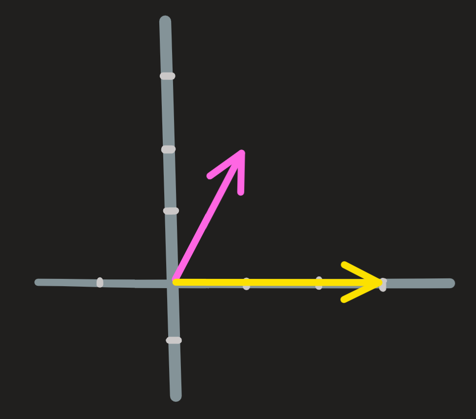
From the picture, it is easy to convince yourself that any linear combination of two vectors of the plane \(\mathbb{R}^2\) is another vector in \(\mathbb{R}^2\), in particular from the l.c. \(0\begin{pmatrix} 1\\2\end{pmatrix}+0\begin{pmatrix} 3\\0\end{pmatrix}\) we get the origin. Hence we write:
\[ \mathbb{R}^2 = \text{span}\{\begin{pmatrix} 1\\2\end{pmatrix},\begin{pmatrix} 3\\0\end{pmatrix}\} \tag{1}\] Another important way to write this set is to identify the form of its elements, the form of its elements is:
\[ a\begin{pmatrix} 1\\2\end{pmatrix}+b\begin{pmatrix} 3\\0\end{pmatrix} \]
or written more compactly \(\begin{pmatrix} a+3b\\2a\end{pmatrix}\). The set of this elements is
\[ \overbrace{\left[\text{all l.c. of $\begin{pmatrix} 1\\2\end{pmatrix}$ and $\begin{pmatrix} 3\\0\end{pmatrix}$ }\right]}^\text{in english} = \overbrace{\text{span}\{\begin{pmatrix} 1\\2\end{pmatrix},\begin{pmatrix} 3\\0\end{pmatrix}\}=\{\begin{pmatrix} a+3b\\2a\end{pmatrix}\,\,|\,\,a,b\in\mathbb{R}\}}^\text{in math, two ways of saying the same thing}=:\overbrace{\mathbb{R}^2}^\text{nick name} \]
- Consider the vector spaces \(\text{span}\{\begin{pmatrix} -3\\2\end{pmatrix},\begin{pmatrix} 4\\-1\end{pmatrix}\}\) and \(\text{span}\{2\begin{pmatrix} 1\\0\end{pmatrix},\begin{pmatrix} 2\\1\end{pmatrix}\}\). Fill the blank space \(\{\_\_\_\_\_ \,\,|\,\, a,b\in\mathbb{R}\}\).
- Now lets do the other way around and from the two forms of the elements \(\begin{pmatrix} a-b\\a+b\end{pmatrix}\) and \(\begin{pmatrix} 3b\\-a+3b\end{pmatrix}\) write the corresponding vector spaces as \(\text{span}\{\_\_\_, \_\_\_\}\).
The idea of a set of things (in this case column vectors) where any l.c. of its elements gives us again an element of the set (we say the set is closed under l.c.) is very important and will appear countless times in this course (note that there are sets where this does not happen, see ….). Hence we give it a special name: vector space.
Definition 1 [Vector space] := a set of vectors with the property of being closed under linear combinations
\(\mathbb{R}^2\) is a vector space.
There are sets which are not closed under linear combinations, see example below
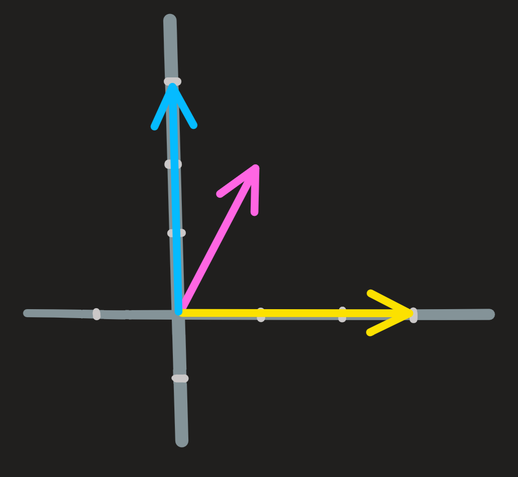
Notice the space \(\mathbb{R}^2\) comes about if we consider \(\begin{pmatrix} 1\\0\end{pmatrix}\) and \(\begin{pmatrix} 0\\1\end{pmatrix}\) as our starting vectors. More, any other pair of vectors of \(\mathbb{R}^2\) that point in distinct directions do the job. Hence we write
\[ \mathbb{R}^2 = \text{span}\{\begin{pmatrix} 1\\2\end{pmatrix},\begin{pmatrix} 3\\0\end{pmatrix}\} = \text{span}\{\begin{pmatrix} 1\\0\end{pmatrix},\begin{pmatrix} 0\\1\end{pmatrix}\}=\cdots \]
Provide another example of vectors \(\mathbf{u}\) and \(\mathbf{v}\) such that:
\[ \mathbb{R}^2=\text{span}\{\mathbf{u},\mathbf{v}\} \]
- Draw this pair of vectors.
- Write the form of the elements of \(\mathbb{R}^2\).
- Why are there so many forms for the elements of \(\mathbb{R}^2\).
- Use the picture above and check \(\begin{pmatrix} 1\\1\end{pmatrix}\in \mathbb{R}^2\) is true.
Example 2
Consider the vector \(\begin{pmatrix} 1\\2\end{pmatrix}\), this is our starting point. Now imagine multiplying it by every possible scalar; the end result is a set of vectors which lie along the same line:
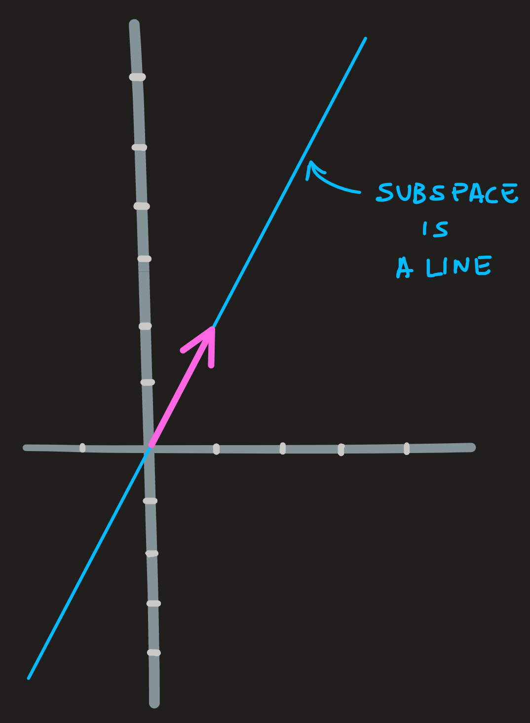
From the picture, it is easy to convince yourself that any linear combination of two (or more) vectors of the line gives us another vector in the line.
\[ \overbrace{\textbf{line}}^\text{nick name} = \overbrace{\text{span}\{\begin{pmatrix}1\\2 \end{pmatrix}\}=\{(a,2a)\,\,|\,\, a\in\mathbb{R}\}}^\text{in math, two ways of saying the same thing} \tag{2}\]
In particular if you multiply any of its vectors by \(0\), we get the origin \(\begin{pmatrix} 0\\0\end{pmatrix}\). Thus the line we are referring passes through the origin and we can say \(\mathbf{0} \in \textbf{line}\).
Once again, since the line is a set closed under l.c., it is a vector space.
Additionally, notice that the line lives inside the plane \(\mathbb{R}^2\), because of that we say it is a subspace of \(\mathbb{R}^2\).
Definition 2 [subspace (of a vector space \(A\))] := a vector space which is a subset of \(A\).
(A subspace is also closed under linear combinations of its vectors.)
Note that: the same line we see in the picture also results if you consider as your starting vector, the vector \(\begin{pmatrix} 2\\4\end{pmatrix}\), and then multiply it by all possible numbers (i.e. all l.c. of this vector). Thus this line can be created in many ways:
\[ \textbf{line} = \text{span}\{\begin{pmatrix}1\\2 \end{pmatrix}\} = \text{span}\{\begin{pmatrix}2\\4 \end{pmatrix}\}=\cdots \]
And the form of its elements are many, such as: \(\begin{pmatrix}a\\2a \end{pmatrix}\), \(\begin{pmatrix}2a\\4a \end{pmatrix}\), \(\dots\)
Fill the blank spaces using your own example \(\mathbf{line}=\text{span}\{\_\_\_\_ \}=\{\_\_\_\,\,|\,\,a\in \mathbb{R}\}\).
Use the picture above to decide which the following statements
\(\begin{pmatrix}-1\\-2 \end{pmatrix}\in \mathbf{line}\)
\(\begin{pmatrix}5\\9 \end{pmatrix}\in \mathbf{line}\)
\(-\begin{pmatrix}2\\4 \end{pmatrix}+\begin{pmatrix}-1\\-2 \end{pmatrix}\in \mathbf{line}\)
are True or False.
- Multiplying a vector by a scalar like we see in the line example is just the linear combination:
\[ a\begin{pmatrix}1\\2\end{pmatrix}+b\begin{pmatrix}0\\0\end{pmatrix} \]
- Any two vectors on the line are parallel, i.e., they are proportional. When two vectors \(\mathbf{u}\) and \(\mathbf{v}\) are proportional we write \(u||v\). For example \(\begin{pmatrix}1\\2 \end{pmatrix}||\begin{pmatrix}2\\4 \end{pmatrix}\), because \(\begin{pmatrix}2\\4 \end{pmatrix}=2\begin{pmatrix}1\\2 \end{pmatrix}\), that is they are proportional with constant \(2\).
- Exercise: Check pictorially whether \(\begin{pmatrix}-1\\2 \end{pmatrix}||\begin{pmatrix}5\\-10 \end{pmatrix}\) and \(\begin{pmatrix}1\\1 \end{pmatrix}||\begin{pmatrix}1\\2 \end{pmatrix}\) are true or false statements.
Example 3
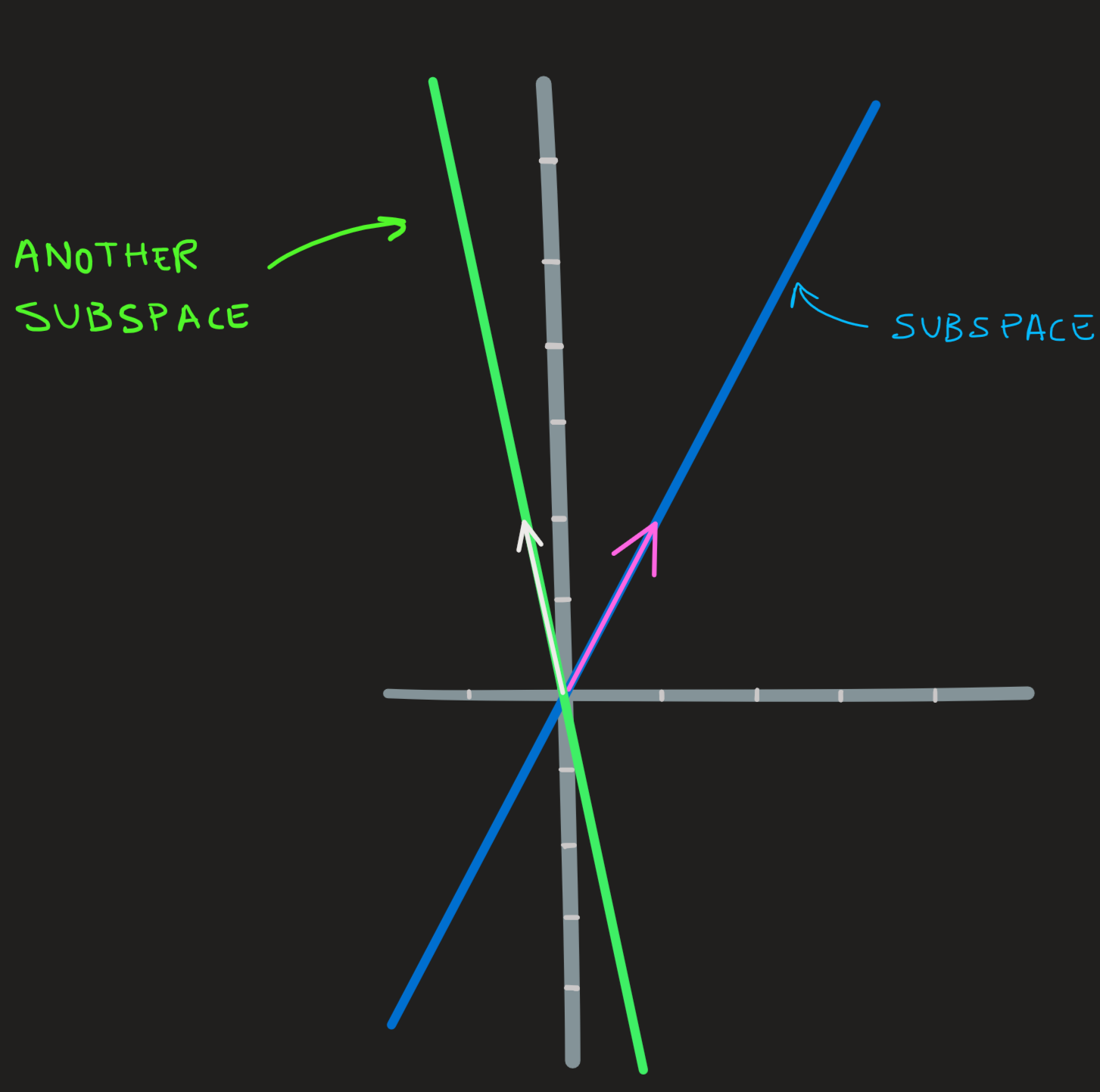
In this example we have show to subspaces of \(\mathbb{R}^2\), the one seen in example 2:
\[ \textbf{line 1} = \text{span}\{\begin{pmatrix}1\\2 \end{pmatrix}\} \]
and now another subspace:
\[ \textbf{line 2} = \text{span}\{\begin{pmatrix}-1/2\\2 \end{pmatrix}\} \]
The origin \(\begin{pmatrix}0\\0 \end{pmatrix}\) belong to both spaces and is the only vector which is common!
An important observation is that by picking one vector of line 1 and another from line 2 we can reach any vector of \(\mathbb{R}^2\), for example the yellow vector is a result of combining the white and pick vectors
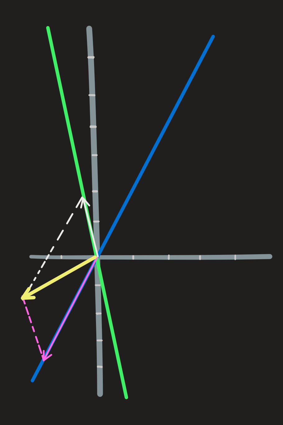
Thus:
\[ \textbf{yellow} = \textbf{white} + \textbf{pink} \]
There not another combination of vectors living in line 1 and line 2 that yield the yellow vector, the combination is unique!
We can now see that any vector in \(\mathbb{R}^2\) can be written, uniquely, as a linear combination of a vector picked from line 1 and another from line 2.
Example 4
Consider the vectors \((1,2,0)^\intercal\) and \((1,0,1)^\intercal\) and \((0,0,1)^\intercal\). Linear combine them with every scalar and you obtain a set of vectors. All these vectors fill the three dimensional space \(\mathbb{R}^3\).
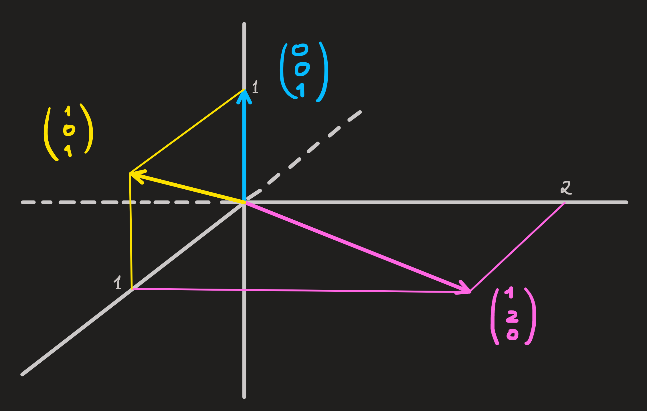
In math notation we write:
\[ \mathbb{R}^3 = \text{span}\{(1,2,0)^\intercal,(1,0,1)^\intercal,(0,0,1)^\intercal\} \]From the picture we can identify some subspaces of \(\mathbb{R}^3\):
\[ [\textbf{pink-blue plane}] = \text{span}\{(1,2,0)^\intercal, (0,0,1)^\intercal\}=\{(a,2a,b)^\intercal\,\,|\,\,a,b\in\mathbb{R}\} \tag{3}\]
\[ [\textbf{xy plane}] = \text{span} \{(1,0,0)^\intercal,(0,1,0)^\intercal\}=\{(a,b,0)^\intercal\,\,|\,\,a,b\in\mathbb{R}\} \tag{4}\]
\[ [\textbf{yellow line}] = \text{span} \{(1,0,1)^\intercal\}=\{(a,0,a)^\intercal\,\,|\,\, a\in\mathbb{R}\} \tag{5}\]
Two important observation regarding these subspaces:
Observation 1: The vector space \(\mathbb{R}^3\) results from summing vectors from the x0y plane and z axis subspaces. Thus any vector in \(\mathbb{R}^3\) can be written as a sum of a vector from the first plus one of the second. We have special notation for this:
Definition 3 Assume we have two subspaces \(U\) and \(W\) of \(\mathbb{R}^3\) (eg. the x0y plane and z axis) where the only common element is the origin \(\mathbf{0}\). Then any vector \(\mathbf{r}\) in \(\mathbb{R}^3\) can be written by some appropriate sum of \(\mathbf{u}\) and \(\mathbf{w}\):
\[ \mathbf{r} = \mathbf{u}+\mathbf{w} \]
In math language:
\[ \mathbb{R}^3 = \{\mathbf{u}+\mathbf{v}\,\,|\,\, \mathbf{u}\in U \,\,\text{and} \,\,\mathbf{v}\in V\} \]
The nick-name of this set is: \(U\oplus V\). The direct sum. Reading \(\mathbb{R}^3=U\oplus V\) from right to left we see what we said above; reading from left to right we see the space being decomposed in subspaces, clearly this can be done in many ways:
\[ \mathbb{R}^3 = [\textbf{xy plane}] \oplus [\textbf{0z line}] = [\textbf{yellow line}]\oplus [\textbf{plane perpendicular to yellow line}]=\cdots \]
In particular the example 3 we could have written:
\[ \mathbb{R}^2= \textbf{line 1} \oplus \textbf{line 2} \]
Observation 2: Let \(A\) and \(B\) be two (non parallel) planes containing the yellow-line, then the intersection of both yields the yellow line:
\[ [\textbf{yellow line}] = A \cap B \]
This is important because it tells us that interception of vectors spaces yields new vector spaces.
As we’ll see later, the interception of two planes is the geometric view of a system with two equations.
Observe the vector \(\begin{pmatrix} 0\\0\\1\end{pmatrix}\) in the picture above.
Does the z-axis constitute a vector space?
Does the positive z-axis constitute a vector space?
Fill the blank: \(\mathbb{R}^3 = \_\_\_ \oplus \textbf{z-axis}\).
Example 5
Consider the vectors \(\begin{pmatrix} 1\\2\end{pmatrix}\) , \(\begin{pmatrix} 3\\0\end{pmatrix}\) and \(\begin{pmatrix} 0\\1\end{pmatrix}\). All linear combinations of these three vectors always yield a vector in \(\mathbb{R}^2\), a two-dimensional vector space and not three-dimensional!
Notice one of the three vectors is redundant.
\[ \mathbb{R}^2 = \text{span}\{\begin{pmatrix} 1\\2\end{pmatrix},\begin{pmatrix} 3\\0\end{pmatrix},\begin{pmatrix} 0\\3\end{pmatrix}\}=\text{span}\{\begin{pmatrix} 1\\2\end{pmatrix},\begin{pmatrix} 3\\0\end{pmatrix}\} \]
In general a vector space \(\mathbb{V}\) is a set of things with which remains invariant under linear combinations. Those things are what we call vectors. A vector is simply a member of this set. An array of numbers, like a column vector, is such an example; matrices, functions are other examples as we’ll see later.
The vector space \(\mathbb{R}^3\) is equal to?
\(A=\text{span}\{\begin{pmatrix}2\\0\\0\end{pmatrix},\begin{pmatrix}1\\2\\0\end{pmatrix},\begin{pmatrix}0\\0\\1\end{pmatrix}\}\)
\(B=\text{span}\{\begin{pmatrix}2\\0\\0\end{pmatrix},\begin{pmatrix}0\\1\\0\end{pmatrix},\begin{pmatrix}1\\2\\0\end{pmatrix},\begin{pmatrix}-3\\1\\0\end{pmatrix}\}\)
\(C=\text{span}\{\begin{pmatrix}1\\0\\0\end{pmatrix},\begin{pmatrix}0\\1\\0\end{pmatrix},\begin{pmatrix}1\\1\\0\end{pmatrix},\begin{pmatrix}0\\0\\2\end{pmatrix},\begin{pmatrix}1\\0\\1\end{pmatrix}\}\)
Is it a vector space?
Example 3 (cont)
Equation 3, Equation 4 and Equation 5 constitute vector spaces because the picture says so. These three equations just express the vector spaces we observed. Imagine, now, we did not have the picture, and our starting point are Equation 3, Equation 4 and Equation 5; how would we know they constitute vector spaces?
Whether they do or do not form vector spaces is a matter of checking the definition of space and apply it to the three equations. Recall the definition: a space is a collection of things which remain invariant under l.c. Lets apply this to Equation 3, the pink-blue plane. Starting from
\[ \{(a,2a,b)^\intercal\,\,|\,\, a,b\in\mathbb{R}\} \tag{6}\]
and without the picture, how would we know this set of \((a,2a,b)^\intercal\) constitute a vector space?
Lets check whether a l.c. of two arbitrary elements of this set is also an element of the set. Hence pick the elements \((a_1,2a_1,b_1)\) and \((a_2,2a_2,b_2)\), these two elements are arbitrary because the numbers \(a_1\) and \(a_2\) are arbitrary. Now take a generic l.c.
\[ \alpha(a_1,2a_1,b_1)+\beta(a_2,2a_2,b_2) \tag{7}\]
It is arbitrary, because the numbers \(\alpha\) and \(\beta\) are also arbitrary, just like the \(a_1\) and \(a_2\) are.
Is Equation 7 an element of that set Equation 6? If it is, Equation 7 must have the form \((a,2a,b)\). Lets check this:
\[ \alpha(a_1,2a_1,b_1)+\beta(a_2,2a_2,b_2) = (\alpha a_1+\beta a_2,2(\alpha a_1 +\beta a_2),\alpha b_1+\beta b_2) = (\spadesuit,2\spadesuit,\clubsuit) \]
It has!
Because, the chosen elements and the l.c. were arbitrary we can conclude that this set is closed under l.c. and therefore constitute a vector space.
Use the same strategy as above to check that Equation 4 and Equation 5 are indeed vector spaces.