Atomic Polynomials
The simplest polynomial involve procedures of the form \(1\), \(x\), \(x^2\), \(x^3\), etc. These functions are given by
\[ \begin{align} e_n:\,\, \mathbb{R} &\longrightarrow\mathbb{R}\\x &\longmapsto e_n(x):= x^n \end{align} \tag{1}\]
for an integer \(n\) of our choice. The function Equation 1 can also be given under the relation notation by:\[ E_n:= \{(x,y)\in\mathbb{R}^2\,\,|\,\, y=x^n\} \tag{2}\]
The graphical version of these functions for \(n=0,1,2,3\) is:
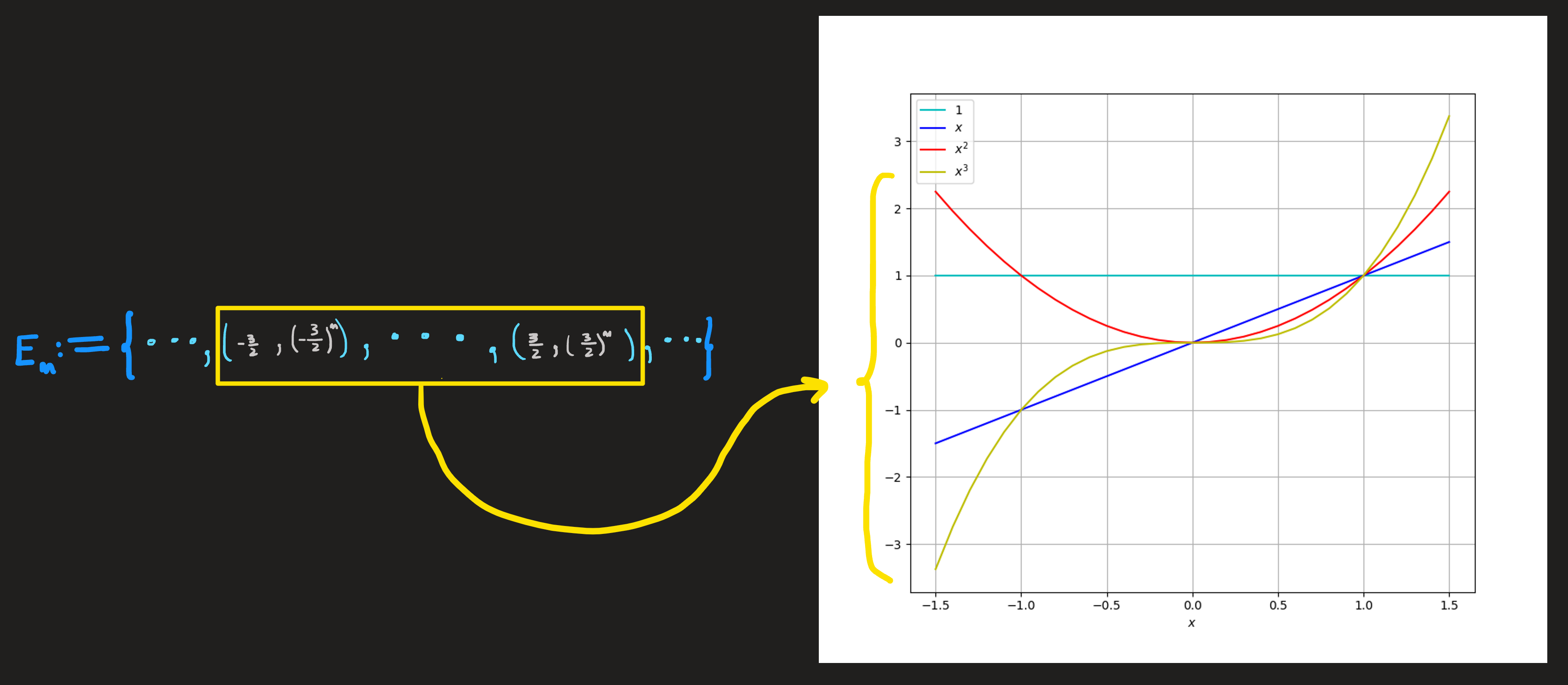
The graph shows the slice of the functions \(E_n\) where \(x\) runs from \(-1.5\) up to \(1.5\) and not the whole function, which according to Equation 1 or Equation 2 has the domain ranging on all reals \(\mathbb{R}\). The slice was chosen because it exhibits interesting part of the function: the region where it intercept the axes (the zeros of the function) and shows maxima/minima.
Properties of the atomic polynomials
Rather than showing a picture of a small slice of the function as de did in Figure 1 we can instead zoom into some aspects of it.
Properties of the connectivity between domain and codomain:
- Range: From inspection of Equation 1 (or Equation 2) we know the domain and codomain of these four functions is \(\mathbb{R}\). The range of these functions is the image of the domain under the action of the function, we can infer what this image is by inspecting Figure 1, for example, the image of \(\mathbb{R}\) under the action of \(e_2\) is the set of all positive reals as we check by the red curve hence we write \(e_2(\mathbb{R})=\mathbb{R}^+_0\). Similarly we find:
\[ e_0(\mathbb{R})=\{1\} \qquad e_1(\mathbb{R})=e_3(\mathbb{R})=\mathbb{R}\qquad e_2(\mathbb{R})=\mathbb{R}^+_0 \]
Onto: We also observe that for even powers of \(n\) such as \(e_0\) and \(e_2\), not all elements in the codomain \(\mathbb{R}\) are hit by outputs, i.e., these are not onto function; as an example, [is \(0\) hit by some \(e_0(x)\) ? Is \(-1\) hit by \(e_2(x)\), for some \(x\) in its domain?] We can answer these question by trying to solve the equations \(e_0(x)=0\) and \(e_2(x)=-1\). To no avail! Neither have solutions \(x\) in the domain \(\mathbb{R}\).
1-1: Additionally nor are these even powers 1-1. Why? Because we can clearly see from Figure 1 that \(e_0\) is in fact the worst possible “labeller”, where all “fruits” \(x\) have exactly the same label \(1\), no other “label” in its codomain \(\mathbb{R}\) is put into good use by this \(e_0\); the function \(e_2\) is not as bad since for each label we find just two elements in \(\mathbb{R}\). The functions \(e_1\) and \(e_3\) are 1-1 since each element \(x\) in their domain have a unique element \(y\) in the codomain, hence if we choose a label \(y\) we uniquely know the \(x\). Summarizing:
\[ \begin{cases}e_0 \qquad &\text{worst possible labeler (one label for all inputs)}\\e_2 \qquad &\text{bad labeller (one label for each pair of inputs)}\\e_1\,\, \text{and}\,\, e_3 \qquad &\text{perfect (one label, one input)}\end{cases} \]
Properties at interesting regions of the function:
Who is bigger or smaller? The Figure 1 reveals something funny:
for points on the horizontal axis close to the origin, that is \(-1<x<1\), the outputs of the four functions have the following rank \(x^3 < x^2 < x^1 < x^0\);
precisely at \(x=1\) we find they are all the same \(x^0=x^1=x^2=x^3=1\);
meanwhile for the remaining points, those in the region \(x<-1 \lor 1<x\), the absolute value of these functions follow the reversed rank! \(x^0<x^1<x^2<x^3\).
For \(x\) very far from \(1\) we find \(x^0\ll x^1\ll x^2\ll x^3\), which means, for example, that \(|x^3|\) is much, much, much, much larger then \(|x^2|\), and so on.
In summary:
\[ \begin{cases} x^3 < x^2 < x^1 < x^0 \qquad &\text{for $x$ close to 1}\\x^0=x^1=x^2=x^3 \qquad &\text{for $x=1$}\\x^0\ll x^1\ll x^2\ll x^3 \qquad &\text{for $x$ far from $1$} \end{cases} \tag{3}\]
This summary will be important when we study the limiting behavior of molecular polynomials.
Zeros: The zeros of a function are the coordinates of the points which intercept the axes. Observing Figure 1 we see polynomial \(1\) intercepts the y-axis at \((0,1)\) while all other polynomials intercept the x-axis and y-axis exactly at the origin \((0,0)\).
Maxima and minima: By inspection of Figure 1, we observe the polynomials \(1\) has no maxima or minima, it is always flat; \(x\) and \(x^3\) on the other hand is a ramp, a never ending one, and thus also does not have a maximum or minimum. The only function exhibiting a minimum is \(x^2\), coincidentally, at \((0,0)\). Only when we study derivatives we’ll have the computational means to find these extrema.
The previous list of properties was already embedded in Figure 1 (or if you think about it, already at Equation 2), only by close observation we made it explicit. Of course, the list is not exhaustive, many other properties remain hidden in that picture, waiting to be dug out. This is why I said this list are a zoom into the picture, when we get closer we see more detail.
As additional examples we could also ask how fast a polynomial of degree one increases, i.e., what is its slope; for polynomials of degree two it would make sense to ask if it its graph is a cup or a cap, it all depends on \(a_2\) parameter.
We usually do not list the properties just as we did above, we just acknowledge in our mind that they exist and compute them as needed, since many times some of them are so bluntly obvious just by looking at the graph or the function formula, that no need is required for a calculation.