Focus-diretrix formulation
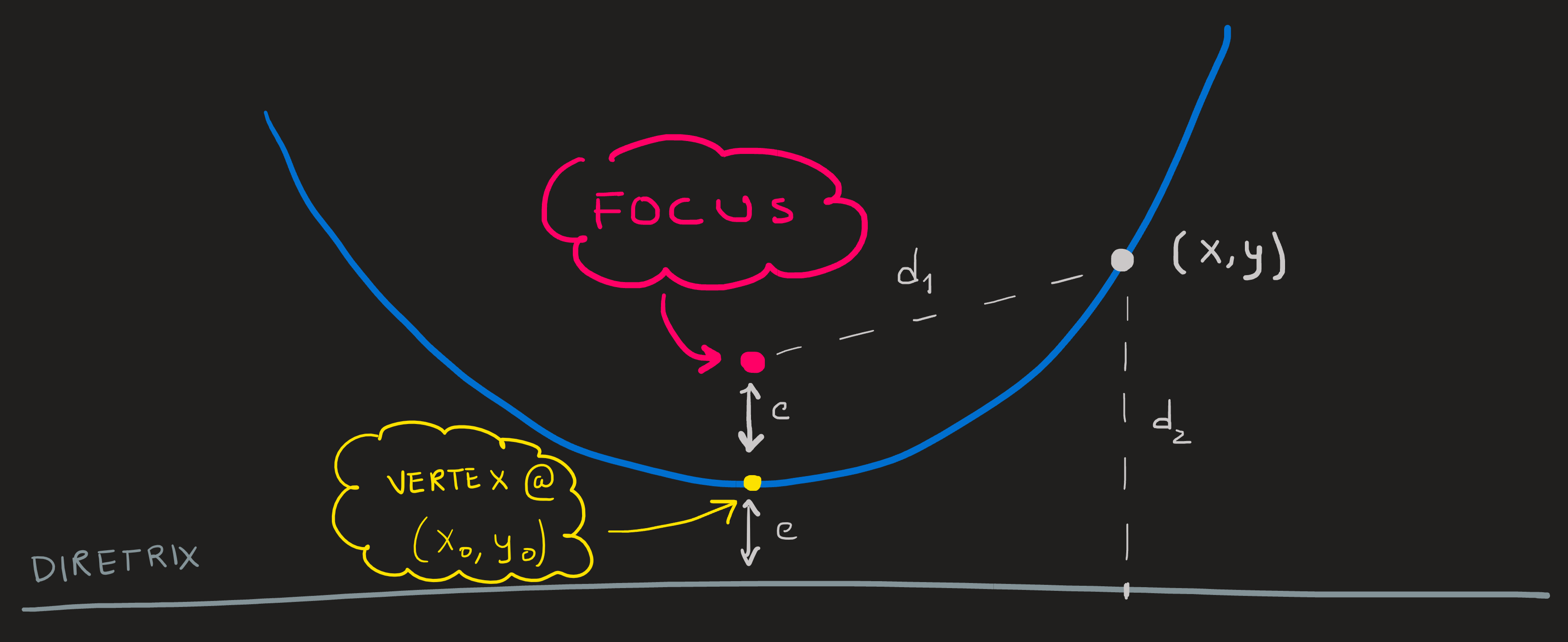
Observing Figure 1 we observe two points: the vertex with coordinates \((x_0,y_0)\) and the focus \(c\) units above at \((x_0,y_0+c)\). A parabola is by definition the set of points which:
Contain the vertex;
A point \((x,y)\) is in the parabola if
[distance from \((x,y)\) to focus] = [vertical distance from \((x,y)\) to diretrix]
The diretrix is the horizontal line \(c\) units below the vertex, as shown in Figure 1 .
When \(c>0\) the polynomials describes a cup whose minimum is the vertex; when \(c<0\) it describes a cap whose maximum is the vertex.
Lets express condition 1. and 2. using mathematical notation.
Using the distance formula we seen above, we can express both distances in terms of the coordinates of the vertex and focus points as
\[ \begin{cases}d_1^2=(x-x_0)^2+(y-(y_0+c))^2\\d_2^2=(y-(y_0-c))^2\end{cases} \]
Condition 2. becomes:
\[ \begin{align} &(x-x_0)^2+(y-(y_0+c))^2 =(y-(y_0-c))^2\\ \iff &(x-x_0)^2+y^2-2(y_0+c)y+(y_0+c)^2 = y^2-2(y_0-c)y+(y_0-c)^2\\ \iff &(x-x_0)^2+y^2-2(y_0+c)y+y_0^2+2y_0c+c^2 = y^2-2(y_0-c)y+y_0^2-2y_0c+c^2\\ \iff&(x-x_0)^2-4cy+4y_0c=0\\ \iff&y=y_0 + \frac{1}{4c}(x-x_0)^2 \end{align} \]
Comparing such calculation with the mediatrix equation we see that the diretrix distance \(d_2\) does not have terms involving \(x\) which guarantees that no cancellation of the \(x\) terms in \(d_1\) thereby preserving its power of \(2\), essential for a polynomial of degree \(2\).
This is the element-hood test for the points in the parabola allowing us describe the set the parabola as the set of pairs
\[ \begin{equation}P_2:= \{(x,y)\,\,|\,\,d_1=d_2\}=\{(x,y)\,\,|\,\,y-y_0=\frac{1}{4c}(x-x_0)^2\}\end{equation} \tag{1}\]
Using the procedure point of view we write:
\[ \begin{equation}\begin{split}p_2:\,\, &\mathbb{R}\longrightarrow \mathbb{R}\\&x \longrightarrow p_2(x):= \frac{1}{4c}(x-x_0)^2+y_0\end{split}\end{equation} \tag{2}\]
These formulas are equivalent to ?@eq-poldeg2, the difference lies in what the parameters mean! While in ?@eq-poldeg2, the \(a_0\), \(a_1\) and \(a_2\) are just the weights of \(1\), \(x\) and \(x^2\); in Equation 1, the \(x_0\) and \(y_0\) are the vertex point of the function and \(c\) is distance from the focus. An analogous situation occurred in polynomials of degree one when we introduced the mediatrix equation.
Zeros of these polynomials:
We wish now to zoom into polynomials given as Equation 1 or Equation 2 and see the zeros of these function are expressed in term of the diretrix and focus properties.
To find vertical axis interception is to find the point \((x,y)\) in \(P_2\) whose \(x=0\):
\[ \begin{equation}\begin{cases}y-y_0=\frac{1}{4c}(x-x_0)^2\\x=0\end{cases}\implies y-y_0=\frac{1}{4c}(0-x_0)^2\implies y=\frac{1}{4c}x_0^2+y_0\end{equation} \]
which tells us the interception point coordinates \((0,\frac{1}{4c}x_0^2+y_0)\) belonging to \(P_2\).
When seeking for the points with \(y=0\) we must be more careful since they may not exist (the parabola might be completely above the x-axis). By substituting again \(y=0\) in the element-hood test we get:
\[ \begin{equation}\begin{cases}y-y_0=\frac{1}{4c}(x-x_0)^2\\y=0\end{cases}\implies(x-x_0)^2=-4cy_0\end{equation} \]
We must be careful when solving for \(x\) the later equation since we must have a positive right hand side, this is only possible if the parameter \(y_0\leq 0\). This is the condition for the existence of zeros, i.e., it is the condition that ensures us the parabola is not completely above the x-axis.
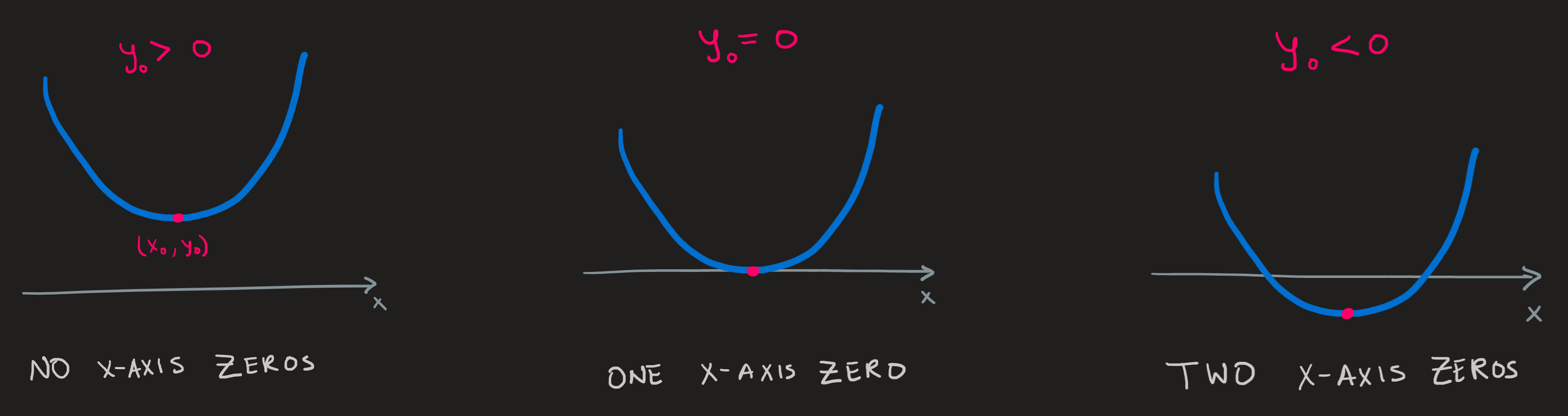
Saying \(y_0\leq 0\) either means, \(y_0=0\), in which case we immediately know \(x=x_0\) and thus \((x_0,0)\) is the ONLY horizontal axis interception (the vertex sits exactly at the x-axis); or it means \(y_0<0\), in this case we solve the equation for \(x\) as follows
\[ \begin{equation}\begin{split}(x-x_0)^2&=4c|y_0|\\&\implies x-x_0=\pm\sqrt{4c|y_0|}\\&\implies x=x_0\pm \sqrt{4c|y_0|}\end{split}\end{equation} \]
There are two interception, at \((x_0+ \sqrt{4c|y_0|},0)\) and another at \((x_0-\sqrt{4c|y_0|},0)\), which is expected when part of the parabola is below the x-axis.
When \(x\) is large:
To understand the behavior when \(x\) is very large, the extreme ends of \(P_2\), we have to note the following:
Observe the term \((x-x_0)^2\), it is a squared of a number \(x-x_0\), hence always positive. This implies the smallest value it takes is zero.
When \(c\) is positive, then \((x-x_0)^2/4c\) is positive for any \(x\), the minimum is zero when we set \(x-x_0=0\).
The procedure \((x-x_0)^2/4c+y_0\) results from the addition of a strictly positive number \((x-x_0)^2/4c\) to \(y_0\), hence the minimum value it can take is \(y_0\) when \(x=x_0\).
Now let us turn into what happens with the function when \(x\) becomes very large (\(x\longrightarrow \pm\infty\)). Another glance at the procedure tell us that the quantity \((x-x_0)^2\) becomes very large either way, multiplying it now by \(1/4c\) we must be clear about the sign of \(c\). If it is positive the function will grow without end in either case, if \(c\) is negative, it becomes very small.
Different formulations of the same procedure
We can rewrite further the expression for the \(p_2(x)\) procedure by expanding the second power
\[ (x-x_0)^2=x^2-2x_0x+x_0^2 \]
Hence \(p_2(x)\) is rewritten as \(p_2(x)=x^2-2x_0x+x_0^2 +y_0\), collecting factors of the same power we have:
\[ \begin{equation}\begin{cases}p_2(x)=a_2x^2+a_1x+a_0\\a_0:= y_0-\frac{x_0^2}{4c}\\a_1:= -\frac{x_0}{2c}\\a_2:=\frac{1}{4c}\end{cases}\end{equation} \]
which clearly shows the highest power of \(x\) is two and hence the classification of degree two.
The coefficients \(a_0\), \(a_1\) and \(a_2\) are determined from the parameters \((x_0,y_0)\) and \(c\), we can if we wish to go the other way around and write how \(x_0\), \(y_0\) and \(c\) are determined from the knowledge of \(a_1\), \(a_2\) and \(a_3\):
\[ \begin{equation}\begin{cases}p_2(x):=(x-x_0)^2+y_0\\x_0:=-\frac{a_1}{2a_2}\\y_0:=\frac{4a_0a_2-a_1^2}{4a_2}\\c:=\frac{1}{4a_2}\end{cases}\end{equation} \]
The two formulation are the same operation but expressed with different leading parameters. All different formulations are distinct in what parameters show up in the expressions, our choice of a formulation essentially is the choice of the parameters that show up.
Going back and forward between formulations is possible at any time, since we have the link between the current \(a_0\), \(a_1\) and \(a_2\) with the \(x_0\), \(y_0\) and \(c\) .