Understanding mapping properties of linear functions
Mapping properties of \(f\)
The way \(f\) maps vectors is analogous to the way \(A\) maps column vectors. Thus, working out properties of the map \(A\) tell us something about the map \(f\). And by properties I mean: is \(f\) 1-1? Onto? Bijective? We can answer these questions by asking them instead to \(A\).
Example 1
Consider two vector spaces whose dimensions are:
\[ \dim \mathbb{V}=3 \qquad \dim\mathbb{W}=1 \]
we do not know what are its elements, but still we label a basis they have as:
\[ \mathbf{B}=(v_1,v_2,v_3)\qquad\mathbf{C}=(w_1) \]
these are just labels, but they immediately tells us that elements of \(\mathbb{V}\) and \(\mathbb{W}\) can acquire the form:
\[ v=\mathbf{B} X \qquad X=\begin{pmatrix}x_1\\x_2\\x_3\end{pmatrix} \tag{1}\]
and
\[ w=\mathbf{C}Y \qquad Y=\begin{pmatrix}y_1\end{pmatrix} \tag{2}\]
I want now to introduce a function \(f:\mathbb{V}\overset{\sim}{\longrightarrow} \mathbb{W}\), but rather than telling a formula for it (which would also require to provide a form for the elements of \(\mathbb{V}\) and \(\mathbb{W}\)) , I decide just to provide the action of \(f\) on the basis labels:
\[ f(v_1)=f(v_3)=2w_1\qquad f(v_2)=0w_1 \]
i.e.
\[ f(\mathbf{B})=\mathbf{C} A \qquad A=\begin{pmatrix}2& 0&2\end{pmatrix} \]
This is enough for us to be able to compute the action of \(f\) on a generic \(v\in\mathbb{V}\):
\[ f(v)=\mathbf{C}AX =\begin{pmatrix} w_1\end{pmatrix} \begin{pmatrix}2& 0&2\end{pmatrix} \begin{pmatrix}x_1\\x_2\\x_3\end{pmatrix} \]
Since we have \(f(v)\in \mathbb{W}\), we know from Equation 2 that \(f(v)=y_1 w_1\), we conclude:
\[ (y_1)=\begin{pmatrix}2& 0&2\end{pmatrix} \begin{pmatrix}x_1\\x_2\\x_3\end{pmatrix} \]
This is \(Y=AX\), mapping the \(v\in \mathbb{V}\) represented wrt \(\mathbf{B}\) into a \(f(v)\) represented wrt \(\mathbf{C}\).
Notice we know how to map any vector even though we did not specify what is \(\mathbb{V}\), nor \(\mathbb{W}\) and neither the form of the basis elements of both, we only provided labels for them. Knowing how \(f\) act on these labels was enough! The reason I am not providing specifics on these sets and on the form of \(f\) is because, they are the bare minimum you need to compute maps; in practice if I have a concrete linear function and sets, I can just easily adapt the above line of reasoning.
The 4 subspaces of a matrix and their consequences
What is the kernel of \(f\)? Adapting the definition to the present example we have to solve the problem of finding the nullspace of the matrix \((2,0,2)\):
\[ AX_N=0 \iff \begin{pmatrix}2& 0&2\end{pmatrix}\begin{pmatrix}x_{1N}\\x_{2N}\\x_{3N}\end{pmatrix}=(0) \]
Since we have one pivot on the first column and two dependent columns, we expect two dimensions.
Isolating \(Col_2\) by setting \(y_N=1\) and \(z_N=0\), the only answer is \(x_N=0\), thus \((0,1,0)^\intercal\) is in the nullspace.
Isolating \(Col_3\) by setting \(y_N=0\) and \(z_N=1\), we find \(x_N=-1\), the second basis vector is \((-1,0,1)^\intercal\).
Any l.c. of these solutions is also mapped to \(0\), thus:
\[ N(A) = span \{(0,1,0)^\intercal,(-1,0,1)^\intercal\} \]
Now we convert the nullspace into the kernel of \(f\) by multiplying the elements of the set by \(\mathbf{B}\) and ?@eq-ker_f:
\[ \ker f = span \{\mathbf{B}(0,1,0)^\intercal,\mathbf{B}(-1,0,1)^\intercal\} \]
The image of \(f\) is \(f(\mathbb{V})\) and we can get it from the column space of the matrix \(A\).
Looking closer at \(AX\) we find:
\[ \begin{pmatrix}2& 0&2\end{pmatrix}\begin{pmatrix}x_{1}\\x_{2}\\x_{3}\end{pmatrix} \]only one independent column, the first one, thus the column space is just:
\[ C(A)=span\{(2)\} \]
And from ?@eq-im_f, the image of \(f\) is:
\[ f(\mathbb{V})=span\{2w_1\} \]
We see that the kernel and image of \(f\) are just analogous to the nullspace and column space of the matrix \((2,0,2)\).
Orthogonal spaces: (Rowspace and left-nullspace) From the matrix \(A\) we can define the row-space as
\[ C(A^\intercal)=span\{(1,0,1)^\intercal\} \]
[Commentary: when multiplied by \(\mathbf{B}\) gives us the image of \(f\). Note that while rowspace and nullspace are orthogonal wrt \(\cdot_{\mathbb{R}^n}\), the corresponding subspaces in \(\mathbb{V}\) need not be, since \(\{v_i\}_{i=1,..,n}\) may not be orthogonal wrt \(\cdot_\mathbb{V}\)]
While the left-nullspace is just
\[ N(A^\intercal)=\{(0)\} \]
The rowspace and nullspace break the domain \(\mathbb{R}^3\) into two subspaces, while the column space and codomain are equal:
\[ \mathbb{R}^3 = span\{(1,0,1)^\intercal\}\oplus span \{(0,1,0)^\intercal,(-1,0,1)^\intercal\}\qquad \mathbb{R} = \mathbb{R}\oplus\{0\} \]
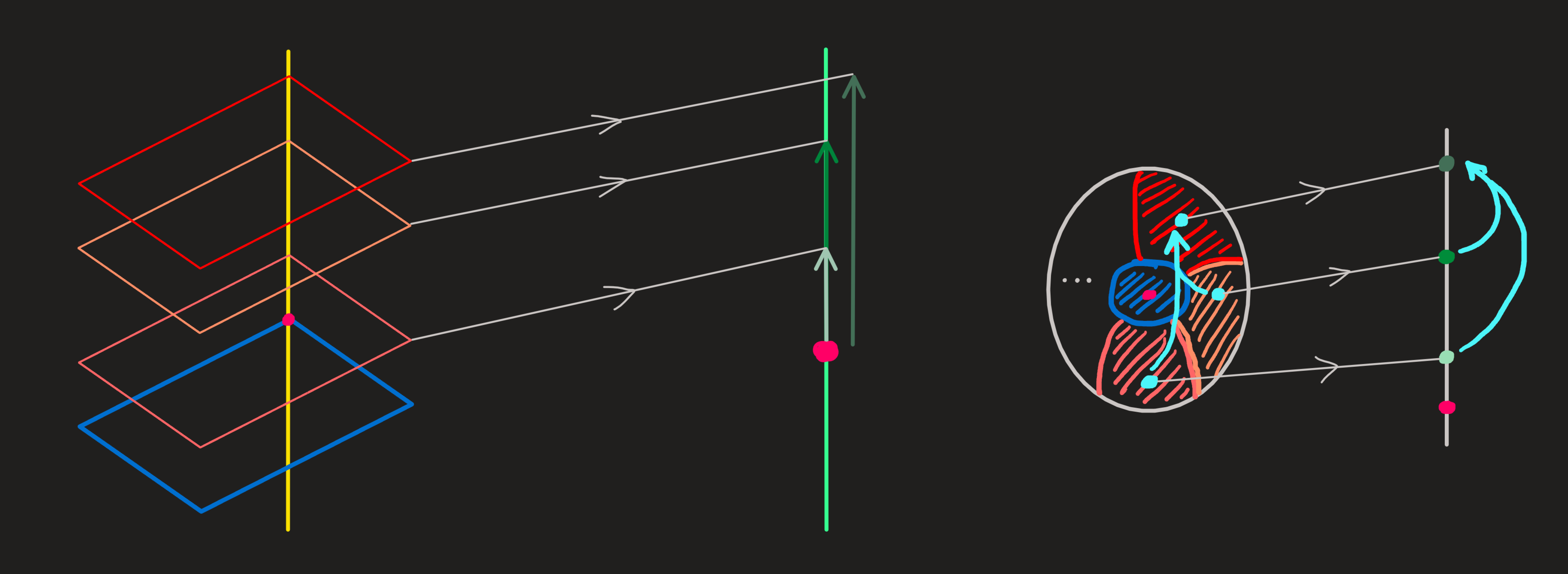
From this, the following picture tells us how one vector \(X\) in \(\mathbb{R}^3\) is mapped into \(AX\in\mathbb{R}\)
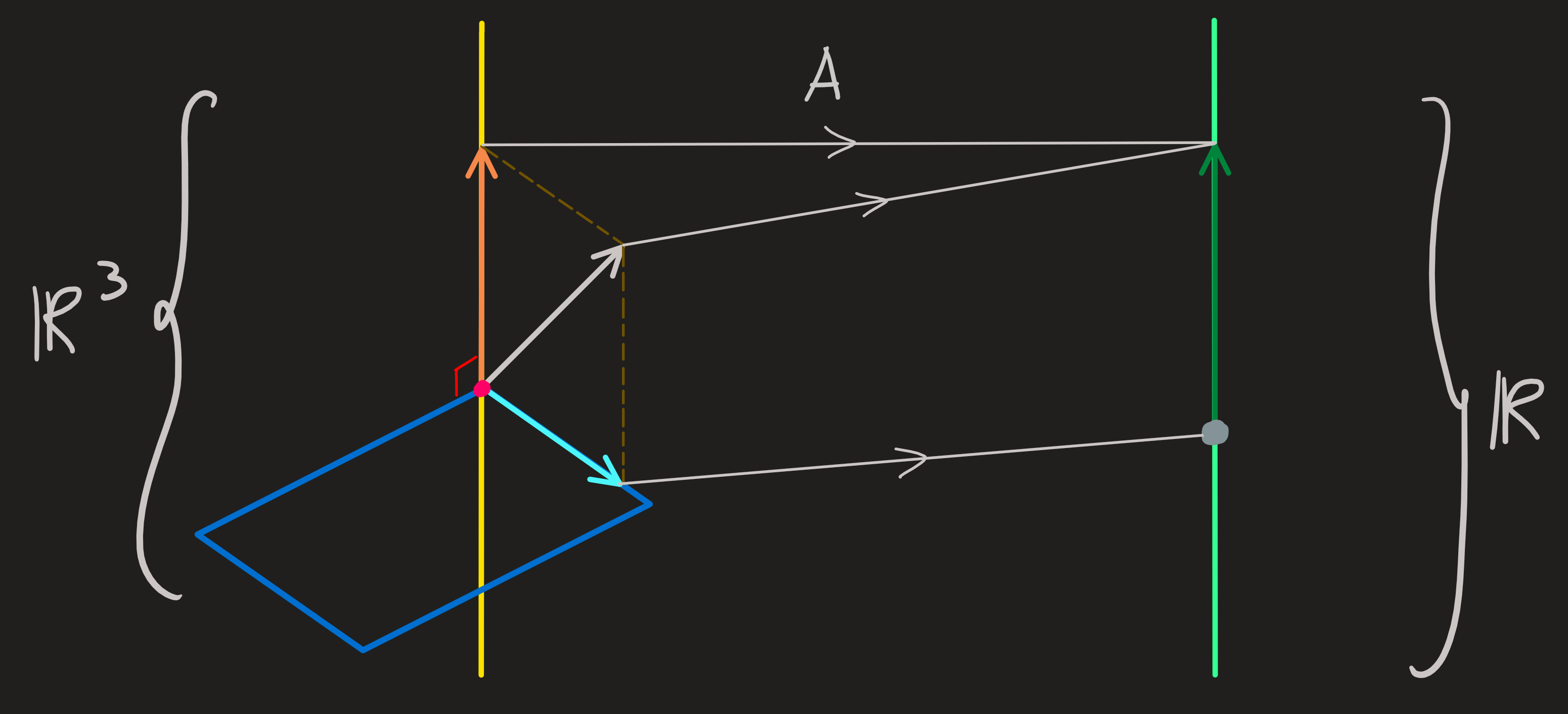
Given these subspaces of the domain and codomain we can now focus on describing the kind of mapping that \(A\) does and turn that \(f\) does. On the picture we see a vector \(X\) being decomposed into its parts, one in the nullspace and another in the row space:
\[ X=X_{R}+X_{N} \]
The \(X_N\) is mapped by this \(A\) into \(0\), and \(X_R\) is mapped into \(AX_R\), thus we can write \(AX=AX_R\) for all \(X\in \mathbb{R}^3\).
For each \(X_R\) in the rowspace we can any add any vector of the null space, the image is always \(AX_R\). Therefore this is not a 1-1 function.
But is it onto? For any element \(Y\) of \(\mathbb{R}\) can we find a \(X\), such that \(AX=Y\) ? I.e. are there always solution \(x_1\) and \(x_3\) such that
\[ y_1=2x_1+2x_3 \]
for any \(y_1\) we choose from \(\mathbb{R}\)? The answer is yes. [Another way to look at this is to notice the \(N(A^\intercal)=\{0\}\)].
Thus \(A\) is onto and so is \(f\).
As a consequence we conclude that any equation
\[ f(v)=w \]
(given a \(w\)) always has solution, in fact has an infinite number of solutions, thanks to the fact that the nullspace is not just \(0\).
Another way to put this, \(f\) has no inverse, however in its place we can define a fiber (a set) as follows:
\[ f^{-1}(w)=\{v\in\mathbb{V}\,\,|\,\,f(v)=w\} \]
To compute this requires solving an already known to us problem \(AX=Y\)! This is what we have been doing in the beginning of the course.
Example 2
Consider two vector spaces \(\mathbb{V}\) and \(\mathbb{W}\) and the following action on a basis:
\[ \begin{align} f(v_1)&=w_1+2w_2+3w_3\\ f(v_2)&=2w_1+4w_2+6w_3\\ f(v_3)&=2w_1+6w_2+8w_3\\ f(v_4)&=2w_1+8w_2+10w_3 \end{align} \]
i.e.
\[ f(\mathbf{B})=\mathbf{C}A,\qquad A=\begin{pmatrix}1 & 2 & 2 & 2 \\2 & 4 & 6 & 8 \\3 & 6 & 8 & 10 \end{pmatrix} \]
The action of \(f\) on some generic element of \(\mathbb{V}\)
\[ v=\mathbf{B}X\qquad X=\begin{pmatrix}x_1\\x_2\\x_3\\x_4\end{pmatrix} \]
is:
\[ f(v)=\mathbf{C}AX=\begin{pmatrix}w_1 & w_2 & w_3\end{pmatrix} \begin{pmatrix}1 & 2 & 2 & 2 \\2 & 4 & 6 & 8 \\3 & 6 & 8 & 10 \end{pmatrix}\begin{pmatrix}x_1\\x_2\\x_3\\x_4\end{pmatrix} \]
And since:
\[ f(v)=\mathbf{C} Y \qquad Y=\begin{pmatrix}y_1\\y_2\\y_3\end{pmatrix} \]
we conclude that:
\[ \begin{pmatrix}y_1\\y_2\\y_3\end{pmatrix}=\begin{pmatrix}1 & 2 & 2 & 2 \\2 & 4 & 6 & 8 \\3 & 6 & 8 & 10 \end{pmatrix}\begin{pmatrix}x_1\\x_2\\x_3\\x_4\end{pmatrix} \]
The nullspace of \(A\) is (we already computed this before, here):
\[ N(A)=span\{\begin{pmatrix}-2\\1\\0\\0 \end{pmatrix},\begin{pmatrix}2\\0\\-2\\1 \end{pmatrix}\} \]
The image of \(f\) is computed from the \(C(A)\), which is:
\[ C(A) =span\{\begin{pmatrix}1\\2\\3\end{pmatrix},\begin{pmatrix}2\\6\\8\end{pmatrix}\} \]
The orthogonal spaces: (rowspace and left-nullspace) Recall the rowspace and left nullspace are orthogonal to these and have the following dimensions:
\[ C(A^\intercal)=span\{(1,2,2,2)^\intercal,(2,4,6,8)^\intercal\} \qquad N(A^\intercal)=span\{(-1,-1,1)^\intercal\} \]
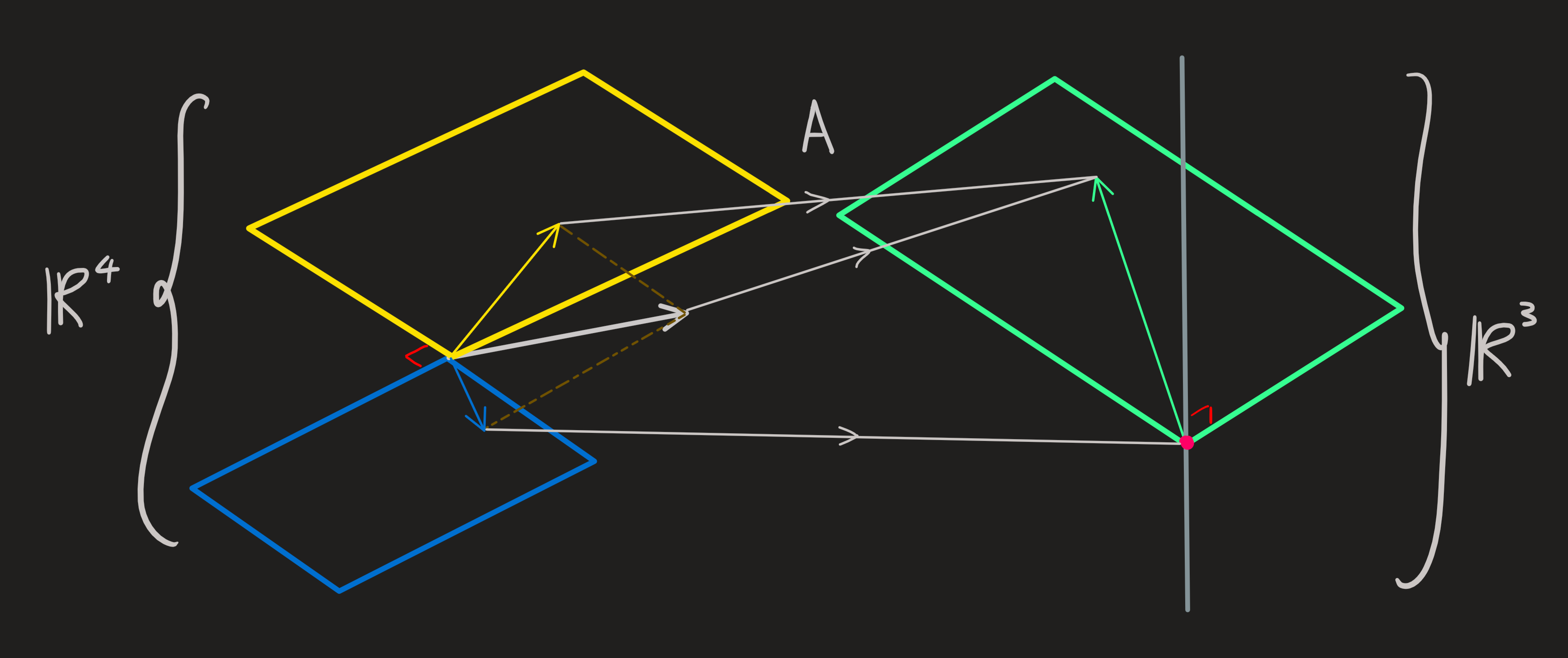
Looking at the diagram, any \(X\), can be broken into two parts:
\[ X=X_R+X_N \]
Any \(Y\) can also be broken into:
\[ Y=Y_C+Y_{LN} \]
The matrix \(A\) maps any \(X\) into the \(C(A)\), the \(N(A^\intercal)\) is never reached. This means that for any \(Y\) with components in the left null space the equation:
\[ AX=Y \]
has no solution.
Any \(Y\) living exclusively in the column space has a fiber of elements of the form \(X_R+X_N\), for a fixed \(X_R\) and \(X_N\) ranging over the entire two dimensional \(N(A)\). [Comment: This \(X_R\) may or not be the particular solution we find when solving a system of equation, see here.]
Evidently, this function is neither 1-1, nor onto, and no inverse (except in the sense of fiber) exists.
Example 3
The map:
\[ \begin{align} f:\mathbb{V}&\longrightarrow \mathbb{W}\\ v&\longmapsto f(v) \end{align} \]
can be specified wrt the bases:
\[ \mathbf{B}=\begin{pmatrix}v_1 & v_2 & v_3\end{pmatrix} \qquad \mathbf{C}=\begin{pmatrix}w_1 & w_2 & w_3\end{pmatrix} \]
by introducing the matrix:
\[ A=\begin{pmatrix}1 & 1 & -1 \\2 & -1& 2 \\1 & 2 & -1\end{pmatrix} \]
Thus \(f(v)\) acquires the form:
\[ f(v)=\mathbf{C}AX \qquad v=\mathbf{B}X \qquad X=\begin{pmatrix}x_1\\x_2\\x_3\end{pmatrix} \]
The map between entries of \(v\) wrt \(\mathbf{B}\) and the entries of \(f(v)\) wrt \(\mathbf{C}\) is the equation:
\[ Y=AX \]
For which we can get the nullspace and column space.
\[ N(A)=\{(0,0,0)^\intercal\} \qquad C(A)=\mathbb{R}^3 \]
just like we computed before.
![]()
There is only one solution. It is 1-1 and surjective. There is inverse.
Example 4:
\[ \begin{align} f:\mathbb{R}^3&\longrightarrow \mathbb{R}^3\\ \mathbf{x}&\longmapsto f(\mathbf{x}):=A\mathbf{x} \end{align} \]
with
\[ A=\begin{pmatrix}2 & -1 \\2 & 1 \\2 & 1\end{pmatrix} \]
The four spaces were already computed before, here is a diagram:
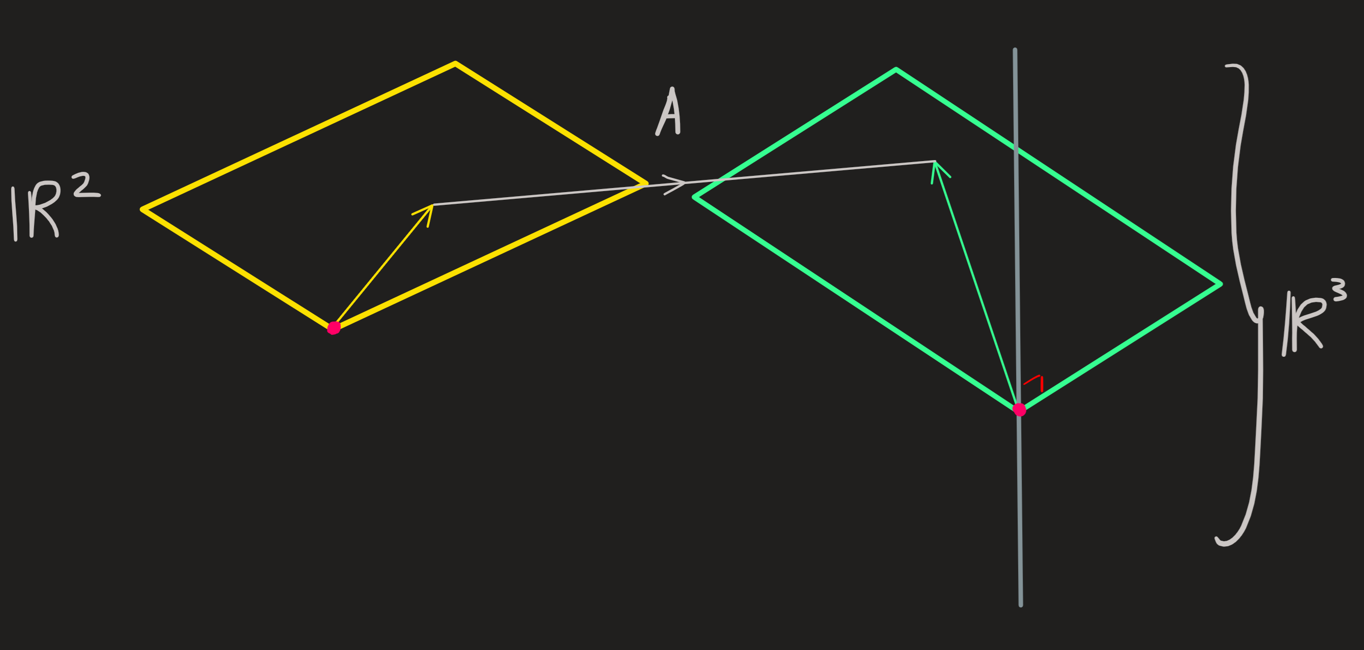
If \(b\) vector is outside column space them there is no solution! Not surjective.
(Mathematical) Motivation: Linear Maps are Structure preserving maps. Whaaaat?
Why are these linear functions important?
The linearity rule says something important about the map \(f\), on the left side of the picture we see a l.c. of elements of \(\mathbb{V}\), i.e., \(\nu u\) and \(\lambda v\) are mapped into \(\nu u+\lambda v\in \mathbb{V}\). This vector in turn is mapped now, under \(f\), into the element \(f(\nu u+\lambda v)\in\mathbb{W}\), see the right side of the picture. Also on the right side we see a l.c. of elements of \(\mathbb{W}\), the element \(f (u)=:u'\) is being combined with the element \(f (v)=:v'\) with the coefficients \(\nu\) and \(\lambda\).
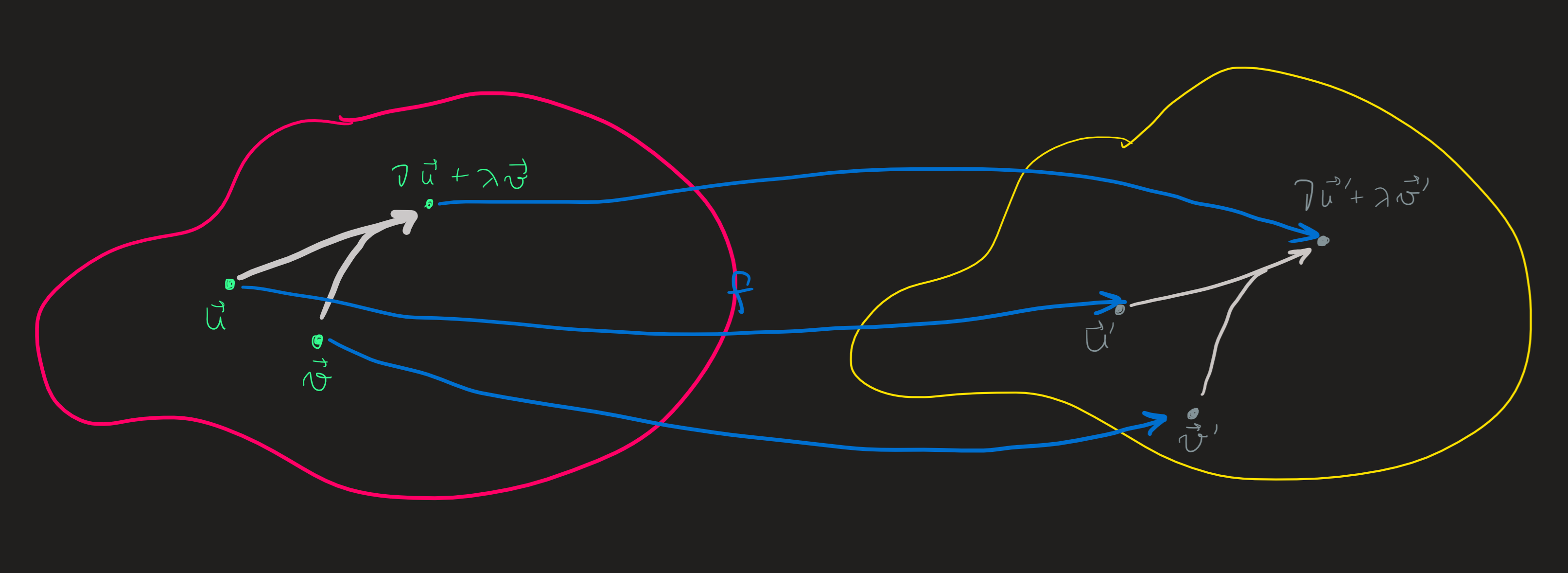
On the picture we see a l.c. diagram-\((\nu,\lambda)\) on the left and another on the right whose coefficients are the same. These diagrams and all the other I did not draw are what we call the connectivity structure of the vector space. Notice, on the left we see the domain of \(f\) and on the right the codomain.
The equality \(f(\nu u+\lambda v) = \nu f (u) + \lambda f(v)\) for coefficients \(\nu\) and \(\lambda\) says the three points of diagram on the left are “connected” to a diagram on the right involving the these same coefficients. The image of the diagram-\((\nu,\lambda)\) on the domain under \(f\) does not change and is reproduced on the codomain.
Lets use the \(f\) from example 1 to illustrate this idea:
If we use two numbers \(\nu\) and \(\lambda\) (eg. \(\nu=\lambda=1\)) to linear combine two vectors of the row space we connected two elements of row space with a third element of the rowspace. This is a concrete example of the diagram on the left side of the picture above.
Acting with \(f\) on the these three we obtain three vectors, which are also connect by a l.c. with the same coefficients (eg. \(\nu=\lambda=1\) we used before).
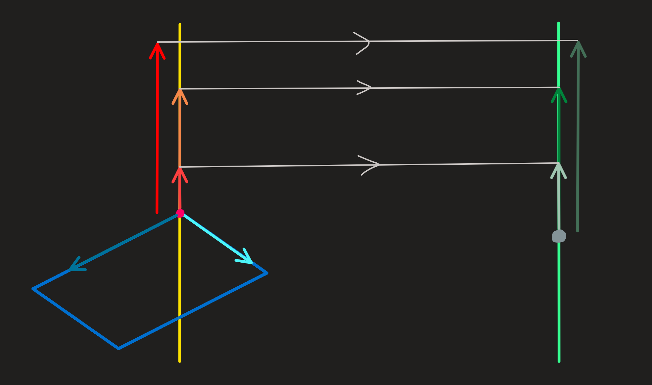
Hence the connectivity we built on the rowspace (=subspace of \(\mathbb{R}^3\)) we reconstituted on the column space.
Now add to each of the chosen vectors in the rowspace the whole nullspace, then any linear combination of vectors of two given planes yield always a vector in the same third plane (eg. combine any dark orange with orange vector and that gives you always a red vector). This is the structure (of connectivity) of the domain. And since the function is linear, these diagrams are replicated in the column space; a light green vector combined with a green vectors yields the same dark green vector.
An example of a non-preserving function is the \(\square\) function
\[ \begin{align}\square:\mathbb{R}^2&\longrightarrow \mathbb{R}^2\\ (x,y)&\longmapsto \square(x,y):=(2x^2,y)\end{align} \]
whose behavior is diagrammatically akin to this:
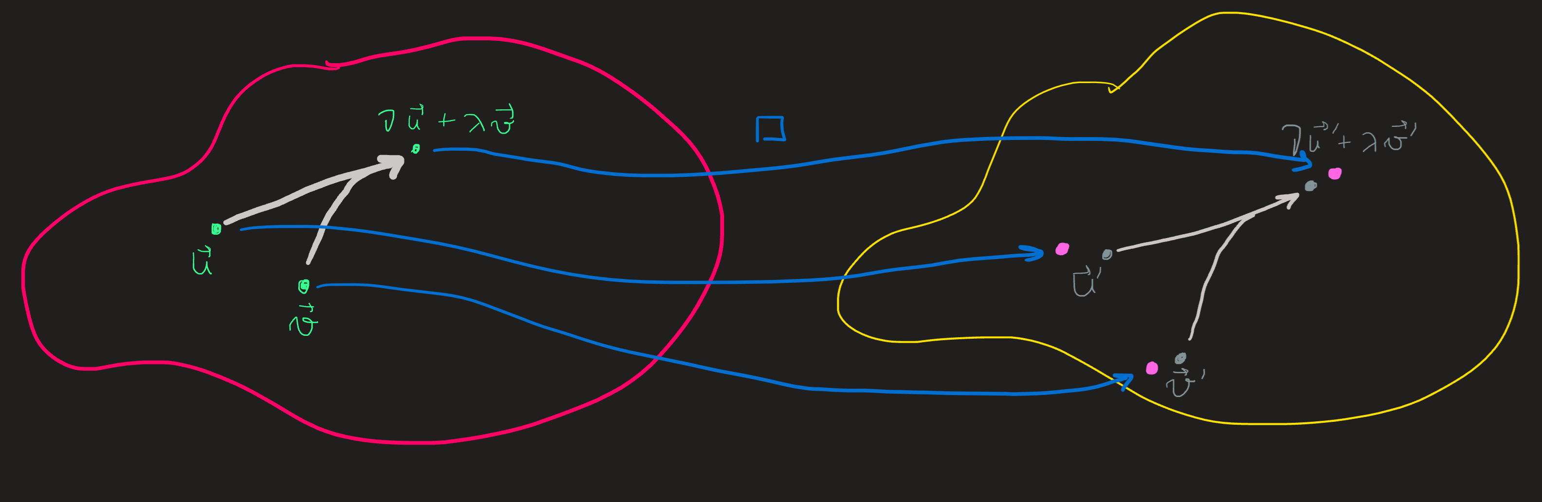
The image of the l.c. diagram on the left does not have a corresponding l.c. diagram (with the same coefficients) on the right. Thus we say \(\square\) does not preserve the diagram during is mapping action.