Matrices
A matrix is simply put an array of numbers with \(n\) rows and \(m\) columns. Here are some examples:
\[ \left(\begin{matrix}1 \\2\\ 100 \end{matrix}\right) \qquad \left(\begin{matrix}1 & 1 & -1\\2 & -1 & 2 \end{matrix}\right) \qquad \left(\begin{matrix}1 & 0 & 0\\0 & 1 & 0\\0 & 0 & 1 \end{matrix}\right) \qquad \left(\begin{matrix}1 & 1 \\2 & -1\\0 & 0 \end{matrix}\right) \qquad \left[(-1)^{i+j}\right] \]
What can we do with matrices?
Answer: linear combinations! [Comment: provided their shape is compatible]
But this time we’ll introduce more: matrix multiplication, transpose, inverses, determinants.
Linear combination of matrices (sum of linear functions)
A number times a matrix is the matrix with every entry multiplied by that number:
\[ \lambda\left(\begin{matrix}1 & 0 & 0\\0 & 1 & 0\\1 & 0 & 1 \end{matrix}\right)=\left(\begin{matrix}\lambda & 0 & 0\\0 & \lambda & 0\\\lambda & 0 & \lambda \end{matrix}\right) \tag{1}\]
From Equation 1 we know in general: \(B_{ij}=\lambda A_{ij}\).
Adding two matrices is done entry-wise:
\[ \left(\begin{matrix}1 & 0 & 0\\0 & 1 & 0\\1 & 0 & 1 \end{matrix}\right)+\left(\begin{matrix}1 & 0 & 1\\0 & 0 & 0\\1 & 0 & 1 \end{matrix}\right) =\left(\begin{matrix}2 & 0 & 1\\0 & 1 & 0\\2 & 0 & 2 \end{matrix}\right) \tag{2}\]
From Equation 2 we identify the rule: \(C_{ij}=A_{ij}+B_{ij}\).
A linear combination \(aA+bB\) is thus computed entry-wise with the rule: \(C_{ij}=aA_{ij}+bB_{ij}\).
Matrix Product (composition of linear functions)
Motivation: Consider the following matrix operation:
\[ \begin{pmatrix}1 & 2 & 2 & 2\\2 & 4 & 6 & 8\\3 & 6 & 8 & 10 \end{pmatrix}\overset{l_2' = l_2-2l_1}{\longrightarrow}\begin{pmatrix}1 & 2 & 2 & 2 \\0 & 0 & 2 & 4 \\3 & 6 & 8 & 10 \end{pmatrix} \]
and corresponding vector operation
\[ \begin{pmatrix} 1\\2\\3 \end{pmatrix} \overset{l_2' = l_2-2l_1}{\longrightarrow} \begin{pmatrix} 1\\0\\3 \end{pmatrix} \]
the operation arrow operator \(\overset{l_2' = l_2-2l_1}{\longrightarrow}\) can be recast as a matrix multiplication:
\[ \begin{pmatrix}1 & 0 & 0 \\-2 & 1 & 0 \\0 & 0 & 1 \end{pmatrix}\begin{pmatrix}1 & 2 & 2 & 2 \\2 & 4 & 6 & 8 \\3 & 6 & 8 & 10\end{pmatrix} = \begin{pmatrix}1 & 2 & 2 & 2 \\0 & 0 & 2 & 4 \\3 & 6 & 8 & 10 \end{pmatrix} \]
and
\[ \begin{pmatrix}1 & 0 & 0 \\-2 & 1 & 0 \\0 & 0 & 1 \end{pmatrix}\begin{pmatrix}1\\2\\3\end{pmatrix}=\begin{pmatrix}1\\0\\3\end{pmatrix} \]
How do we do these calculations?
The general rule is:
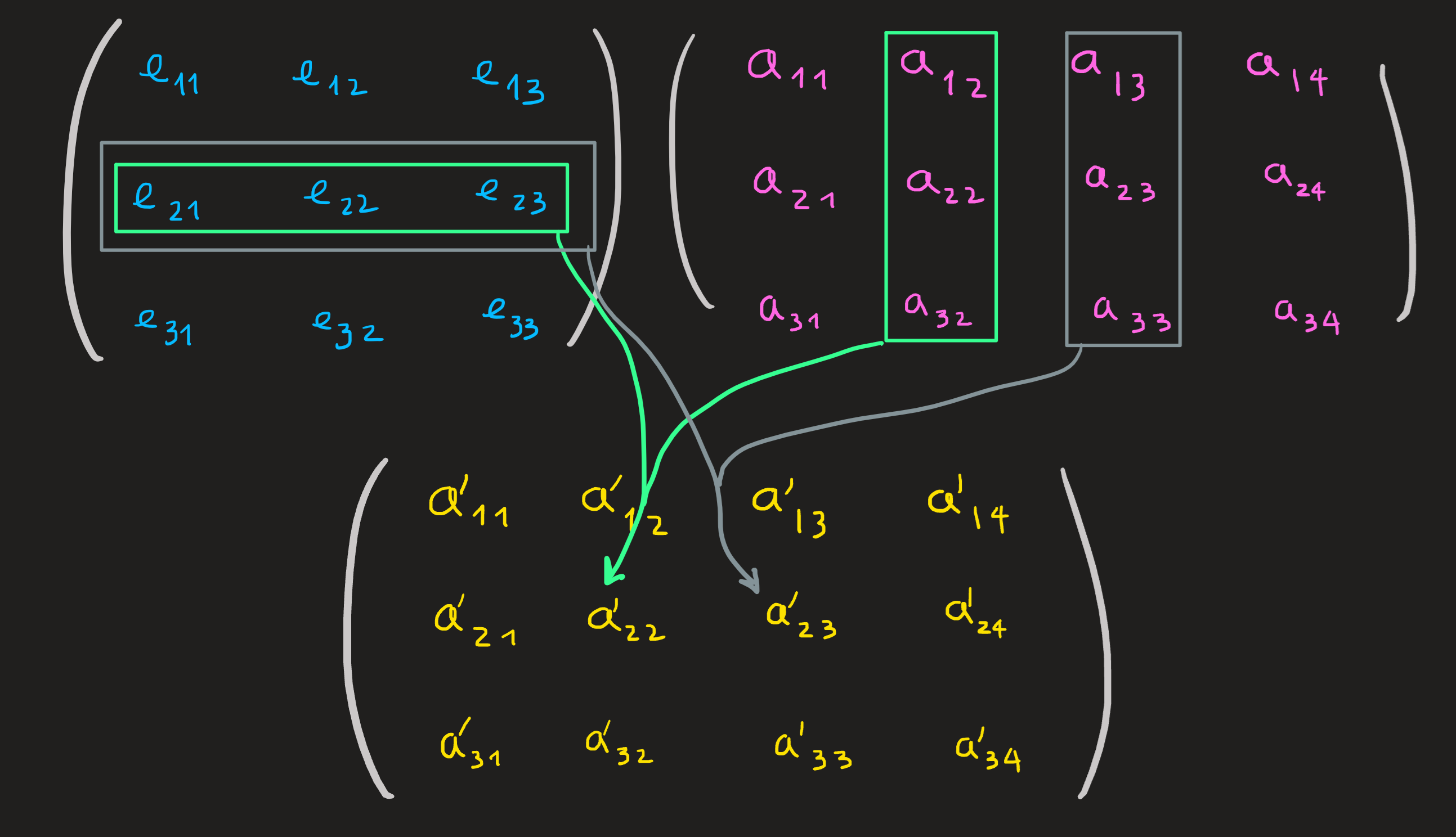
where, for example:
\[ \begin{align} a_{22}'= e_{21}a_{12} + e_{22}a_{22} +e_{23}a_{32}\\ a_{23}'= e_{21}a_{13} + e_{22}a_{23} +e_{23}a_{33}\\ \end{align} \]
Lets name the matrices involved, the \(e\)’s matrix is called \(E_1\) and the \(a\)’s matrix is called \(A\), the result of the multiplication is called \(A'\).
Another way to put it, is to see the first column of \(A'\) is the l.c. of the columns of \(E\) with coefficients of the first column of \(A\); yet another way is to note the first row of \(A'\) as the l.c. of rows of \(A\) with coefficients on the first row of \(E\).
Observing Figure 1 and ?@eq-ex_of_mm we see two important aspects about \(E_1 A\)
The shape of \(E_1\) is \(3\times3\), the shape of \(A\) is \(3\times 4\) and the shape of \(A'\) is \(3\times4\).
The matrix \(E_1\) needs to have as many columns as there are rows in \(A\) (in this case \(3\)), otherwise it is not possible to do matrix multiplication. In other words, the compatible shapes for matrix multiplication are of the form \([m\times r][r\times n] = [m\times n]\), for any integers \(m,n,r\). For example, the case above is \([3\times 3][3\times 4]\) and thus \(m=3\), \(r=3\) and \(n=4\).
The general formula for the entries of \(A'\) is the complicated formula:
\[ a_{ij}'=\sum_{k=1}^re_{ik}a_{kj} \]
Transpose
The transpose of a matrix \(A\) is the operation of turning its rows into a column, for example:
\[ \begin{pmatrix}1 & 2 & 2 & 2\\2 & 4 & 6 & 8\\3 & 6 & 8 & 10 \end{pmatrix}^\intercal = \begin{pmatrix}1 & 2 & 3 \\2 & 4 & 6 \\2 & 6 & 8 \\2 & 8 & 10 \end{pmatrix} \]
In components: \((A^\intercal)_{ij} =A_{ji}\).
Properties: (which can be verified with basic examples)
\((A^\intercal)^\intercal=A\)
\((A+B)^\intercal=A^\intercal+B^\intercal\)
\((AB)^\intercal = B^\intercal A^\intercal\)
Component rules of complicated matrix operations
Example 1:
We want to compute the entries of the matrix \(AB-BA\) in terms of the entries of the matrices \(A\) and \(B\).
\[ (AB)_{ij} = \sum_k A_{ik}B_{kj} \qquad (BA)_{ij} = \sum_k B_{ik}A_{kj} \]
Thus:
\[ (AB-BA)_{ij} = (AB)_{ij} - (BA)_{ij} = \sum_k A_{ik}B_{kj} - \sum_k B_{ik}A_{kj}=\sum_k (A_{ik}B_{kj} -B_{ik}A_{kj}) \]
Example 2:
Compute all matrices that commute (\(AB-BA=0I\)) with the matrix \(A_{ij}=1\) with \(i,j=1,2\).
We see the solution \(B\) for the problem:
\[ 0=\sum_{k=1,2} (A_{ik}B_{kj} -B_{ik}A_{kj}) \]
Since the entries of \(A\) are all ones this equation reduces to:
\[ 0=\sum_{k=1,2}(B_{kj}-B_{ik}) \iff 0= B_{1j}+B_{2j}-B_{i1}-B_{i2} \iff B_{1j}+B_{2j}=B_{i1}+B_{i2} \]
In words: \(B\) must be in such a way what, the sum of the entries in any of its columns must be the sum of the entries in any of its rows. After some guess work we arrive at the general form for \(B\):
\[ \left(\begin{matrix}\alpha & \beta \\\beta & \alpha \end{matrix}\right) \]
Exercises: 2.1.All